Redis Deep Dive Part 2 - The Building Blocks

This is the second post in our Redis internals series. In the previous blog, we looked at the event loop model of Redis and how it makes Redis so fast even with a single thread. In this post, we’re going to examine the basic data structures of Redis.

What you’ll learn:

• How Redis organizes data internally
• Why Redis uses multiple encodings for the same data type
• How to choose the right data structure for your use case

📌 Version Note: This post covers Redis 7.x primarily. Key differences: Redis 7+ uses listpack instead of ziplist. For Redis 6.x, substitute ziplist for listpack throughout.

---

From Database to Dictionary

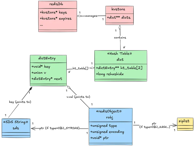
First of all, imagine Redis as a database. Somehow, Redis has to be represented in the code; that representation is redisDb. The redisDb structure contains a kvstore pointer that holds all key-value pairs. (This kvstore in turn manages the underlying hash tables, or dicts). It also has other fields to make some actions faster and safer, such as key eviction and managing concurrent operations.

typedef struct redisDb {
   /* The keyspace for this DB. As metadata, holds keysizes histogram */
    kvstore *keys;  
    /* Timeout of keys with a timeout set */           
    kvstore *expires;
    /* Hash expiration DS. Single TTL per hash (of next min field to expire) */
    ebuckets hexpires;
    /* Keys with clients waiting for data (BLPOP)*/          
    dict *blocking_keys;        
    /* Keys with clients waiting for data, 
       and should be unblocked if key is deleted (XREADEDGROUP). 
       This is a subset of blocking_keys*/
    dict *blocking_keys_unblock_on_nokey; 
    dict *ready_keys;           /* Blocked keys that received a PUSH */
    dict *watched_keys;         /* WATCHED keys for MULTI/EXEC CAS */
    int id;                     /* Database ID */
    long long avg_ttl;          /* Average TTL, just for stats */
    unsigned long expires_cursor; /* Cursor of the active expire cycle. */
} redisDb;

Why does this matter? Every Redis command you execute - whether it’s GET, LPUSH, or ZADD - ultimately interacts with this keyspace. Understanding how this system works is key to understanding Redis performance.

Before going further, as you can see, Redis stores the key-valie pair in a kvstore, ultimately in a dictionary. When storing the key space in the dictionary a common practice called hashing is used. Keys are converted into hashes using a hash function, and the hashes are distributed into buckets for easy access.

Since future keys are usually unpredictable, it is hard to determine the optimal size of the buckets at the start. So, either:

1. We over-allocate and waste storage.
2. We under-allocate and experience collisions.

To avoid this, Redis uses two techniques, namely:

1. Chaining, which allows multiple keys to be stored in the same bucket by linking them in a list. However, it’s important to ensure that chains don’t become too long, as this can degrade the hash table’s performance.
2. Rehashing, which redistributes the keys when the chain length exceeds a certain threshold. Rehashing can be costly, but Redis mitigates this with progressive rehashing, which spreads the rehashing process over time.

Now let’s check the Key value Store (_kvstore) structure.

struct _kvstore {
    int flags;
    dictType dtype;
    dict **dicts;
    long long num_dicts;
    long long num_dicts_bits;
    /* List of dictionaries in this kvstore that are currently rehashing. */
    list *rehashing;                       
    /* Cron job uses this cursor to gradually resize dictionaries 
    (only used if num_dicts > 1). */
    int resize_cursor;                     
    int allocated_dicts;                   /* The number of allocated dicts. */
    int non_empty_dicts;                   /* The number of non-empty dicts. */
    unsigned long long key_count;          /* Total number of keys in this kvstore. */
    /* Total number of buckets in this kvstore across dictionaries. */
    unsigned long long bucket_count;       
    /* Binary indexed tree (BIT) that describes cumulative 
    key frequencies up until given dict-index. */
    unsigned long long *dict_size_index;   
    size_t overhead_hashtable_lut;         /* The overhead of all dictionaries. */
    size_t overhead_hashtable_rehashing;   /* The overhead of dictionaries rehashing. */
    void *metadata[];                      /* conditionally allocated based on "flags" */
};

The KV store groups keys by dict-index. In cluster mode, Redis uses this to store keys from the same hash-slot together.

Let’s check the Key value Store (dict) structure.

struct dict {
    dictType *type;

    dictEntry **ht_table[2];
    unsigned long ht_used[2];

    long rehashidx; /* rehashing not in progress if rehashidx == -1 */

    /* Keep small vars at end for optimal (minimal) struct padding */
    unsigned pauserehash : 15; /* If >0 rehashing is paused */

    unsigned useStoredKeyApi : 1; /* See comment of storedHashFunction above */
    signed char ht_size_exp[2]; /* exponent of size. (size = 1<<exp) */
    /* If >0 automatic resizing is disallowed (<0 indicates coding error) */
    int16_t pauseAutoResize;  
    void *metadata[];
};

It uses two hash tables (ht[0] and ht[1]) for progressive rehashing. When resizing, Redis migrates data gradually to avoid latency spikes.

How it works: Instead of rehashing all keys at once (which could block Redis for milliseconds), Redis rehashes a small number of buckets during each operation. This means that during a rehash, lookups check both ht[0] and ht[1], while insertions go directly to ht[1].

Below function is used to perform the progressive rehashing,

int dictRehashMicroseconds(dict *d, uint64_t us) {
    if (d->pauserehash > 0) return 0;

    monotime timer;
    elapsedStart(&timer);
    int rehashes = 0;

    while(dictRehash(d,100)) {
        rehashes += 100;
        if (elapsedUs(timer) >= us) break;
    }
    return rehashes;
}

Above function rehashes in 100-bucket increments until a time budget (typically microseconds) is exhausted. This keeps the main thread responsive while gradually completing the rehash.

Now that we understand how Redis manages its dictionaries, let’s examine what they actually store.

From Dictionary to Data

As seen above dictionary holds hash tables of dict_entry, each dictEntry holds a key pointer (which points to an SDS string) and a value union that can hold a pointer to a redisObject (robj).

struct dictEntry {
    struct dictEntry *next;  /* Must be first */
    void *key;               /* Must be second */
    union {
        void *val;
        uint64_t u64;
        int64_t s64;
        double d;
    } v;
};

The union stores small integers directly in the entry, avoiding separate allocations and saving memory.

However, for most data types, the value pointer in dictEntry points to a redisObject (robj), which wraps the actual data structure.

struct redisObject {
    unsigned type:4;           /* Logical data type (String, List, Set, etc.) */
    unsigned encoding:4;       /* Internal representation (List might be quicklist or ziplist)*/
    unsigned lru:LRU_BITS;     /*  Used for memory eviction policies LRU time or LFU data */
    unsigned iskvobj : 1;      /* 1 if this struct serves as a kvobj base */
    unsigned expirable : 1;    /* 1 if this key has expiration time attached */
    unsigned refcount : OBJ_REFCOUNT_BITS;  /* Reference count */
    void *ptr;                 /* Points to actual data structure */
};

This design incurs overhead: each object uses ~16 bytes for the robj header, plus 8-16 bytes for allocator alignment. This is why storing millions of tiny keys can consume surprising amounts of memory.

Memory optimization insight: This overhead is why Redis uses compact encodings like ziplist and intset - they store multiple items in a single robj, amortizing the header cost.

Data Access Flow

How does all this connect when accessing data? When you execute GET mykey, here’s what happens:

1. Redis hashes mykey to find the bucket in ht[0] (or both tables during rehash)
2. Traverses the collision chain to find the matching dictEntry
3. Follows the dictEntry->val pointer to the robj
4. Checks robj->type and robj->encoding to determine how to interpret the data
5. Follows robj->ptr to the actual data structure (SDS, ziplist, etc.)
6. Returns the value to the client

Most Redis operations are O(1) due to hash table lookups. The encoding determines how step 4 retrieves the actual data.

Core Data Structures

This framework—database, dictionary, objects—applies to all Redis data types. But step 4 mentioned ‘encoding,’ and that’s where things get interesting. Let’s explore how Redis actually implements each data type.

Strings (Simple Dynamic Strings - SDS)

Strings are the fundamental building block - even keys in Redis are SDS strings. A custom structure stores length (len), allocated space (alloc), and the character buffer (buf).

typedef char *sds;

/* Modern SDS structures (Redis 3.2+) */
struct __attribute__ ((__packed__)) sdshdr8 {
    uint8_t len;         /* used */
    uint8_t alloc;       /* excluding the header and null terminator */
    unsigned char flags; /* 3 lsb of type, 5 unused bits */
    char buf[];
};

/* ... (sdshdr16, sdshdr32, sdshdr64) ... */

There are 4 different implementations (sdshdr8, sdshdr16, sdshdr32, sdshdr64) optimized for different string lengths. Redis automatically picks the smallest header that can represent the string. The older version (Redis 2.x-3.0) used a simpler but less memory-efficient structure:

/* Legacy SDS structure (Redis 2.x-3.0) */
struct sdshdr {
    int len;        /* Length of occupied space in buf */
    int free;       /* Length of free space remaining in buf */
    char buf[];     /* Data space */
};

The modern version saves memory by using appropriately-sized integer types (uint8_t for strings under 256 bytes, etc.).

Advantages

1. O(1) Length Retrieval

Direct read of len field, no scanning for null terminators like C strings. Commands like STRLEN return instantly, even for multi-megabyte strings. With C strings, you’d need to scan the entire string.

2. Binary Safety

Can store null characters (\0) anywhere because length is tracked explicitly, not calculated from null terminators.

Storing serialized Protocol Buffers, images, or any binary data. Traditional C strings would truncate at the first null byte.

3. Efficient Appends - Pre-allocation Strategy

Redis pre-allocates extra space to reduce frequent reallocations.

Pre-allocation logic,

• When length < 1MB: Redis doubles the allocation (exponential growth)
• When length >= 1MB: Redis adds 1MB extra space (linear growth)

Eg If you’re using APPEND to build a log string:

• First append (10 bytes): Allocates 20 bytes (doubles)
• Second append (now 20 bytes): Allocates 40 bytes
• Continue until 1MB, then allocations grow by 1MB chunks

This means APPEND is amortized O(1) instead of O(n) with naive reallocation.

While strings handle scalar values efficiently, Redis also needs to store ordered collections. Enter lists.

Lists

Quicklist: The modern primary implementation; a doubly-linked list where each node is a ziplist (or listpack in newer versions) segment.

What is a Ziplist?

A ziplist stores all entries in one contiguous memory block instead of allocating separate nodes. This eliminates pointer overhead.

[zlbytes][zltail][zllen][entry1][entry2][entry3]...[zlend]

This saves memory but makes insertions in the middle expensive (requires memmove).

Quicklist: Best of Both Worlds

/* From quicklist.h */
typedef struct quicklist {
    quicklistNode *head;        /* Head of the linked list */
    quicklistNode *tail;        /* Tail of the linked list */
    unsigned long count;        /* Total count of all entries in all ziplists */
    unsigned long len;          /* Number of quicklistNodes */
    int fill : QL_FILL_BITS;    /* Fill factor for individual nodes */
    unsigned int compress : QL_COMP_BITS; /* Depth of end nodes not to compress */
    /* ... */
} quicklist;

/* Each node in the quicklist */
typedef struct quicklistNode {
    struct quicklistNode *prev; /* Previous node */
    struct quicklistNode *next; /* Next node */
    unsigned char *zl;          /* Pointer to ziplist (or quicklistLZF if compressed) */
    /* ... */
} quicklistNode;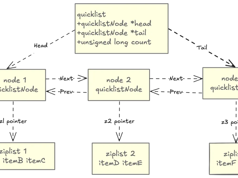

Instead of one giant ziplist (expensive to modify) or a pure linked list (memory overhead), quicklist segments the list into multiple ziplist chunks.

Advantages:

1. Memory Density: Ziplists pack entries tightly in contiguous memory
2. Amortized O(1) Operations: LPUSH, RPUSH, LPOP, RPOP hit the head/tail nodes
3. Fast Sequential Access: Efficient traversal due to cache-friendly memory layout
4. Balanced Design: Avoids large ziplist copy operations by segmenting into nodes

Lists maintain order but allow duplicates. Sets flip this: unordered but unique elements. This different guarantee enables different optimizations

Sets

Sets in Redis use two possible encodings based on content and size.

Encoding 1: intset (for small, integer-only sets)

Implemented as a compact sorted array of integers, very memory efficient.

/* From intset.h */
typedef struct intset {
    uint32_t encoding;  /* INTSET_ENC_INT16, INT32, or INT64 */
    uint32_t length;    /* Number of elements */
    int8_t contents[];  /* Compact sorted array of integers */
} intset;

Features:

• Sorted array of integers (enables binary search)
• Very memory efficient (no pointer overhead)
• Automatically upgrades encoding (int16 → int32 → int64) as needed

Eg: A set containing {1, 5, 100} uses only 3×2 = 6 bytes (as int16) plus header (~8 bytes), totaling ~14 bytes. A hash table implementation would need ~100+ bytes.

Operations:

• Membership test: O(log N) via binary search
• Add/remove: O(N) due to sorted array maintenance
• This trade-off makes sense for small sets (N < 512 by default)

Encoding 2: Hash Table (for large or string-containing sets)

Uses the standard dict hash table (same as the main keyspace), providing O(1) average case add/remove/lookup operations.

When you execute SADD myset 42:

1. Redis checks if myset uses intset encoding
2. If yes and 42 is an integer: Binary search + insert in sorted position (O(N))
3. If set is too large or 42 is a string: Convert to hash table (one-time O(N) cost)
4. All subsequent operations are O(1) average case

Warning: Converting from intset to hash table blocks Redis briefly. Pre-convert large sets or tune the threshold to avoid this.

Hashes

Sets store unordered values; hashes store unordered key-value pairs. Like sets, hashes switch encodings based on size, but they optimize for field lookups rather than membership tests.

Encoding 1: ziplist (or listpack in Redis 7+)

Used for tiny hashes (small number of fields, small field/value lengths), offering high memory efficiency by storing entries contiguously.

Structure:

[field1][value1][field2][value2]...

What is a listpack? (Redis 7+): An improved version of ziplist that:

• Doesn’t require full traversal for some operations
• Has better worst-case performance
• More resilient to fragmentation

Redis 7+ automatically uses listpack where ziplist was used previously.

Encoding 2: Real Hash Table

Redis converts to a standard hash table of dictEntrys once thresholds are exceeded, ensuring lookups remain fast for large hashes.

The “Hash-per-Object” Optimization

Problem: Storing millions of small objects as individual Redis keys:

SET user:1000:name "Alice"
SET user:1000:email "alice@example.com"
SET user:1000:age "30"

Each key wastes memory on overhead: dictEntry, robj header, and SDS key.

Solution: Store as a hash:

HSET user:1000 name "Alice" email "alice@example.com" age "30"

If the hash stays under thresholds, it uses ziplist encoding - one robj header for all three fields.

Memory savings: For 1 million users with 10 fields each:

• Individual keys: ~1GB just in overhead
• Hash encoding: ~100MB in overhead (10× reduction)

Trade-off: You lose per-field expiration and can’t use GET directly. Use HGET instead.

Hashes and regular sets are unordered, giving up ordering for O(1) operations. But what if you need both fast lookups and sorted data? That’s where sorted sets come in.

Sorted Sets (ZSets)

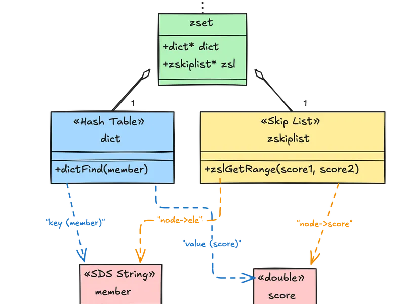
Sorted sets combine two data structures to provide both fast member lookup and efficient ordered traversal.

/* From server.h */
typedef struct zset {
    dict *dict;       /* Hash table: member -> score mapping (O(1) lookup) */
    zskiplist *zsl;   /* Skip list: maintains sorted order (O(log N) range ops) */
} zset;

/* Skip list structure */
typedef struct zskiplist {
    struct zskiplistNode *header, *tail;
    unsigned long length; /* Number of elements */
    int level;            /* Max level of any node */
} zskiplist;

typedef struct zskiplistNode {
    sds ele;                  /* Member (string) */
    double score;             /* Score */
    struct zskiplistNode *backward; /* Backward pointer */
    struct zskiplistLevel {
        struct zskiplistNode *forward;
        unsigned long span;   /* Number of nodes to skip */
    } level[];
} zskiplistNode;

Why Two Structures?

Dual-index design: Redis maintains both structures simultaneously, updating both on every change.

1. Hash Table (dict): O(1) average lookup to check if a member exists or get its score
   • Used by: ZSCORE, ZRANK, ZINCRBY
2. Skip List (zskiplist): O(log N) range queries and ordered traversal
   • Used by: ZRANGE, ZRANGEBYSCORE, ZREVRANGE

Example workflow for ZINCRBY myzset 10 "alice":

1. Hash table lookup: Find alice’s current score (O(1))
2. Skip list deletion: Remove old score node (O(log N))
3. Skip list insertion: Insert new score node (O(log N))
4. Hash table update: Update score in dict (O(1))

Total: O(log N), which is acceptable for the power of ordered operations.

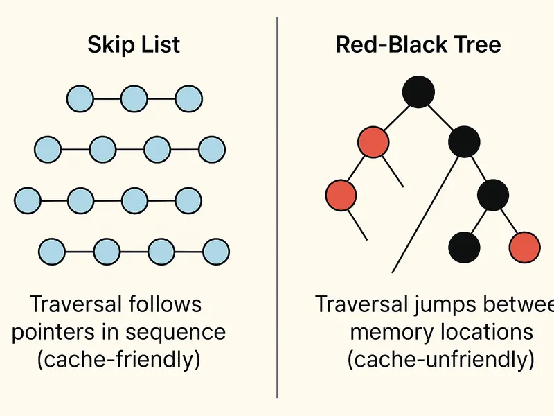
Skip Lists: Why Not Balanced Trees?

Redis chose skip lists over AVL/Red-Black trees for sorted sets. Here’s why:

1. Simpler Implementation

• Skip lists: ~200 lines of straightforward code
• Red-Black trees: ~500+ lines with complex rotation logic

2. Similar Performance

• Both offer O(log N) operations
• Skip lists have simpler constants

3. Better Cache Locality

• Sequential traversal in skip lists follows forward pointers (cache-friendly)
• Tree traversal jumps around memory unpredictably

4. Range Queries

• Skip lists naturally support efficient range queries (follow forward pointers)
• Trees require in-order traversal or threading

Memory layout comparison:

For very small sorted sets (< 128 members), Redis uses ziplist encoding instead of the dual skip list + hash table. This saves memory at the cost of O(N) operations.

We’ve covered Redis’s core collection types—lists, sets, hashes, and sorted sets. Redis 5.0 introduced a new category: Streams, designed specifically for log-style data.

Streams (Redis 5.0+)

Streams are Redis’s log-like data structure, optimized for append-only time-series data.

A radix tree (also called Patricia trie) is a space-optimized prefix tree where nodes with single children are merged. Redis uses it to index stream entries by ID.

Example stream IDs: 1526569495631-0, 1526569495631-1, 1526569498234-0

Radix tree structure:
    "1526569"
        ├─ "495631-"
        │    ├─ "0" → [entry]
        │    └─ "1" → [entry]
        └─ "498234-0" → [entry]

Common prefixes are shared, saving memory.

Uses a radix tree (called Rax) for indexing and listpack structures for the actual entries.

/* From stream.h */
typedef struct stream {
    rax *rax;             /* Radix tree holding the stream entries */
    uint64_t length;      /* Number of elements in stream */
    streamID last_id;     /* Zero if there are no items */
    rax *cgroups;         /* Consumer groups dictionary: name -> streamCG */
} stream;

Why radix tree? Stream IDs have common prefixes (timestamp portion), making radix trees very space-efficient. Random-access by ID is fast (O(log N)), and range queries (XRANGE) are efficient.

Features:

• Log-like data type for event sourcing
• Time-based IDs (timestamp-sequence format: 1526569495631-0)
• Fast insertion (append-only) and range queries by ID
• O(log N) lookup via radix tree
• Consumer groups for distributed processing

Command mapping:

When you execute XADD mystream * field1 value1:

1. Redis generates ID: current timestamp + sequence (Eg: 1526569495631-0)
2. Creates listpack containing [field1, value1, …]
3. Inserts into radix tree with ID as key
4. Updates stream metadata (length, last_id)

Use cases:

• Event logs (clickstreams, audit logs)
• Message queues with consumer groups
• Time-series data (sensor readings, metrics)
• Activity feeds

So far, we’ve looked at data structures that store discrete values or collections. Bitmaps take a different approach: treating strings as bit arrays.

Bitmaps

Bitmaps aren’t an actual data structure in Redis - they’re a specialized way of working with strings at the bit level. This makes them extremely memory-efficient for tracking boolean information across large domains.

Bitmaps leverage Redis strings (SDS) and treat them as arrays of bits. Since strings can be up to 512 MB, bitmaps can address up to 2³² (4,294,967,296) different bits.

Memory layout example:

String value: "\x05\x06\x07"
Bit representation:
Byte 0: 00000101 (bits 0-7)
Byte 1: 00000110 (bits 8-15)
Byte 2: 00000111 (bits 16-23)

Avoid if:

1. Sparse data: If user IDs are 64-bit integers with large gaps (Eg: UUIDs), you’ll waste memory. Solution: Use a hash function to map IDs to a smaller range, or use sets instead
2. Small populations: For fewer than ~10,000 items, sets are often simpler and more flexible
3. Need metadata: Bitmaps only store binary state. If you need timestamps or additional properties, use hashes or sorted sets

Performance characteristics:

• Setting/getting individual bits: O(1)
• Counting bits: O(N) but highly optimized with CPU-level popcount instructions
• Bitwise operations: O(N) where N is string length in bytes

Bitfields

Bitmaps work with single bits. Bitfields extend this: instead of 1-bit flags, you can pack multiple integers of arbitrary bit width (1-64 bits) into the same string. This enables efficient storage of multiple counters or small numeric values.

Like bitmaps, bitfields operate on Redis strings but provide atomic operations for multi-bit integer access.

Redis provides three overflow policies for increment/decrement operations:

1. WRAP (default): Wraps around on overflow

   • 255 + 1 = 0 for unsigned 8-bit
   • 127 + 1 = -128 for signed 8-bit

2. SAT (saturate): Stays at min/max value

   • 255 + 1 = 255 for unsigned 8-bit
   • 127 + 1 = 127 for signed 8-bit

3. FAIL: Returns nil and doesn’t modify

   • Useful when overflow would indicate an error condition

Use bitfields when:

• You need multiple small counters per key (reduces key overhead)
• Values fit in small bit ranges (1-32 bits typically)
• Atomic increment/decrement with overflow control is important
• Memory efficiency is critical

Avoid if:

• Values require more than 64 bits
• You need range queries (use sorted sets instead)
• Access patterns are random (hash tables might be simpler)

Performance characteristics:

• All operations: O(1)
• Atomic even for multiple operations in one command
• Highly memory efficient for small integers

We’ve seen how Redis optimizes storage for flags and counters. Another specialized use case is geographic data, which Redis handles through geospatial indexes.

Geospatial Indexes

Redis geospatial capabilities allow you to store and query geographic coordinates efficiently. Internally, it’s implemented as a sorted set with a clever encoding trick.

Geospatial indexes use sorted sets where the score is a geohash (a 52-bit integer encoding latitude and longitude).

Geohash encoding example:

Coordinates: (37.7749, -122.4194)  // San Francisco
Encoded as: 9q8yyk8yuv6  // Base32 geohash
Stored as: 52-bit integer in sorted set score

Geohashes enable efficient spatial indexing by encoding 2D coordinates into a single sortable value:

1. Hierarchical Spatial Locality

Nearby locations have similar geohash values, allowing range queries on the sorted set:

2. Precision Levels

Longer geohashes = higher precision:

• 1 character: ~5,000 km × 5,000 km
• 3 characters: ~156 km × 156 km
• 5 characters: ~5 km × 5 km
• 7 characters: ~152 m × 152 m

Redis uses 52 bits (~26 characters precision) for sub-meter accuracy.

3. Z-order Curve

Geohash interleaves latitude and longitude bits, creating a space-filling Z-order curve that preserves locality:

Geospatial indexes give exact location queries. But sometimes you don’t need precision—you just need to count unique items efficiently. That’s where HyperLogLog shines.

HyperLogLog

HyperLogLog estimates unique element counts using only ~12KB, regardless of set size.

Redis implements HyperLogLog as a specialized string encoding with statistical counters.

How it works:

1. Hash each element to a 64-bit value
2. Use first 14 bits to select one of 16,384 registers
3. Count leading zeros in remaining 50 bits
4. Store maximum leading zeros count in selected register
5. Estimate cardinality from register values

HyperLogLog provides ~0.81% standard error with 12KB memory:

Register encoding optimization:

Redis uses two encodings for HyperLogLog:

1. Sparse encoding (for small cardinalities < ~10K):

   • Stores only non-zero registers
   • Uses run-length encoding
   • Can be as small as 100 bytes

2. Dense encoding (for large cardinalities):

   • Full 12 KB array of 16,384 registers
   • Redis automatically converts when beneficial

Beyond Core Redis: Redis Stack Extensions

While we’ve covered the fundamental data structures that form the foundation of Redis, there are several specialized data types worth mentioning:

These types are part of Redis Stack (formerly Redis Modules) and not included in core Redis:

1. JSON (RedisJSON)

• Provides native JSON document storage with path-based operations
• Supports complex nested structures and atomic updates
• Use cases: Configuration storage, API responses, document databases

2. Time Series (RedisTimeSeries)

• Optimized for time-stamped data with automatic downsampling
• Built-in aggregation functions (avg, sum, min, max)
• Use cases: Metrics, sensor data, financial ticks

3. Vector Similarity Search (RediSearch)

• Enables AI/ML workloads with vector embeddings
• Supports hybrid search (vectors + structured filters)
• Use cases: Semantic search, recommendation systems, RAG applications

4. Probabilistic Structures (RedisBloom)

Beyond HyperLogLog, includes:

• Bloom Filter: Membership testing with false positive rate
• Cuckoo Filter: Like Bloom but supports deletions
• Count-Min Sketch: Frequency estimation for streaming data
• Top-K: Track K most frequent items

Choosing the Right Data Structure

Data Type	Encoding(s)	Best For	Key Operations	Avg Complexity
Strings	SDS (int/embstr/raw)	Caching, counters, bitmaps	GET, SET, INCR	O(1)
Lists	Quicklist (ziplist nodes)	Queues, stacks, timelines	LPUSH, RPOP	O(1) ends
Sets	intset / hash table	Tags, unique items, voting	SADD, SISMEMBER	O(1) avg
Hashes	ziplist/listpack / dict	Objects, sessions, small docs	HSET, HGET	O(1) fields
Sorted Sets	ziplist / skiplist + dict	Leaderboards, priority queues	ZADD, ZRANGE	O(log N)
Streams	rax + listpack	Event logs, message queues	XADD, XREAD	O(log N) + O(N) range
Bitmaps	String (bit operations)	Boolean flags, analytics	SETBIT, BITCOUNT	O(1) / O(N)
Bitfields	String (int operations)	Compact counters, permissions	BITFIELD	O(1)
Geospatial	Sorted set (geohash)	Location search, proximity	GEOADD, GEORADIUS	O(log N)
HyperLogLog	String (probabilistic)	Cardinality estimation	PFADD, PFCOUNT	O(1)

Try It Yourself:

Experiment with the concepts in this post:

# Clone Redis and explore the source
git clone https://github.com/redis/redis.git
cd redis
# Check out the files mentioned:

# Or use Redis locally to test encodings:
redis-cli

# Create small hash (ziplist)
HSET small field1 "value1" field2 "value2"
OBJECT ENCODING small  # "listpack"

# Create large hash (hashtable)
HSET large $(for i in {1..600}; do echo "field$i value$i"; done)
OBJECT ENCODING large  # "hashtable"

# Test HyperLogLog
PFADD visitors user1 user2 user3
PFCOUNT visitors  # Returns approximate count

# Test Geospatial
GEOADD locations -122.419 37.775 "SF" -118.244 34.052 "LA"
GEODIST locations SF LA km

# Test Bitmaps
SETBIT active:users 100 1
SETBIT active:users 500 1
BITCOUNT active:users

---

Further Reading:

• Redis Source
• Redis Data Types Documentation
• Redis Memory Optimization
• Redis Internals
• HyperLogLog Algorithm Explained
• Redis Geospatial Commands

About this series: This is part 2 of our Redis Internals series. Read part 1 about the Event Loop

---